Project

MATH 490 Project

Author: Michael Volk
Date: 2022.12.13

§ Introduction

Message Passing Framework

Traditionally machine learning over graphs has relied on graph statistics and kernel methods, the idea being to convert the graph in to a representation that can capture high level information about node neighbors and graph structure. These representations could then be used for a prediction task on the graph like a node or graph classification. Graph statistics and kernel methods are limited because they rely on hand engineered features and they don't adapt through the learning process. Additionally the handcrafted engineering of these features can be time consuming on reliant specialist domain knowledge. Instead the representation can be learned.

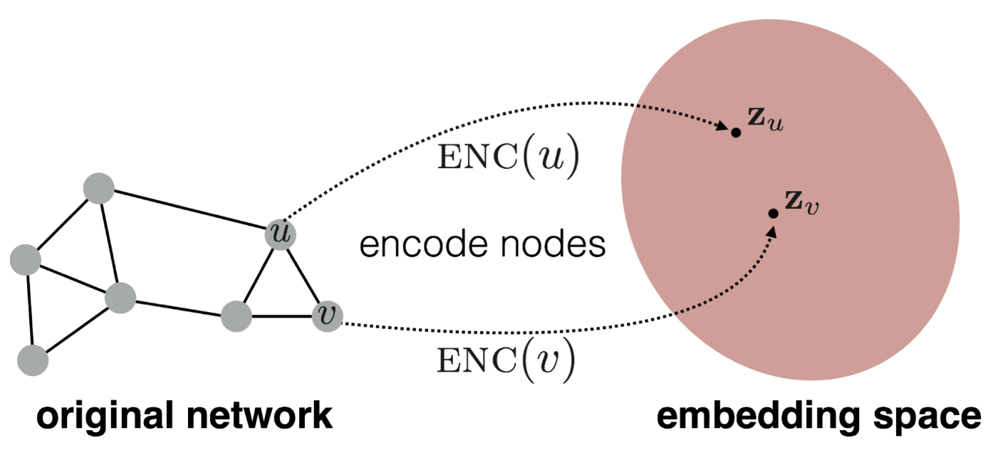
The idea is to learn a mapping from nodes $u$ and $v$ to $z_u$ and $z_v$ (Image¹). A decoder $DEC$ then decodes the embeddings vectors according to a supervised or unsupervised objective. A loss can then be back propagated through the $DEC$ and then the $ENC$ to update model weights. One way to do this is through the message passing framework.

One of the major motivations for the message passing framework is the fact that graph data is non-Euclidean, which precludes graphs from being input to a Euclidean convolutional neural network. The message passing framework generalized the convolution to non-Euclidean data. Furthermore it can be motivated by the color refinement algorithm that is presented in the Weisfeiler-Lehman(WL) graph isomorphism test.

Here we present the message passing framework as presented by the popular PyTorch Geometric Library. This definition of message passing will be used to define the different types of message passing neural networks.

$\mathbf{x}_i^{(k)}=\gamma^{(k)}\left(\mathbf{x}_i^{(k-1)}, \square_{j \in \mathcal{N}(i)} \phi^{(k)}\left(\mathbf{x}_i^{(k-1)}, \mathbf{x}_j^{(k-1)}, \mathbf{e}_{j, i}\right)\right)$
$\square_{j \in \mathcal{N}(i)}$ : Differentiable, permutation invariant function, e.g. sum, mean, or max.

$\phi^{(k)}$ : Differentiable functions such as Multi-Layer Perceptrons (MLPs).

$\gamma^{(k)}$ : Differentiable functions such MLPs.

Toy Example

To gain some intuition of a message passing framework we will take a small graph as example.

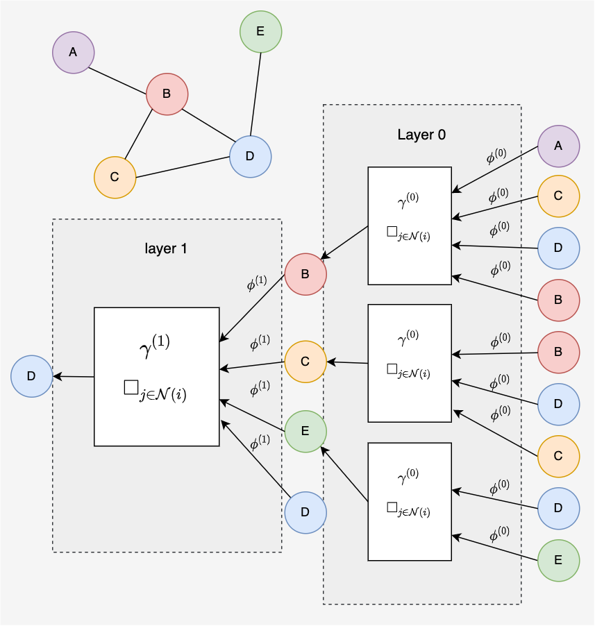
We will consider messages passed to node $D$ in a 2-layer message passing neural network. The computational graph can be traced out from node $D$ first to a 1-hop neighborhood and then to a 2-hop neighborhood. The 1-hop neighborhood contains all nodes except node $A$ . Including node $D$ is often considered optional and is can be interpreted as adding self-loops to the graph. Layer 0 looks shows connections from the 2-hop neighborhood of node $D$ .

Popular Message Passing Neural Networks

Graph Convolutional Neural Network (GCN)

Message Passing View

$\mathbf{x}_i^{\prime}=\boldsymbol{\Theta}^{\top} \sum_{j \in \mathcal{N}(v) \cup\{i\}} \frac{e_{j, i}}{\sqrt{\hat{d}_j \hat{d}_i}} \mathbf{x}_j$
$e_{i,j}$ : edge weight from node $j$ to node $i$ (i.e. with no edge weight, $e_{i,j} = \mathbf{1}$ ).

$\hat{d}_{i} = 1 + \sum_{j \in \mathcal{N}(i)}$ : weighted degree of node $i$ , plus 1 to avoid divide by 0.

$\Theta^{\top}$ : Weight matrix

Matrix View

$X^l = \sigma(\hat{D}^{-1/2}\hat{A}\hat{D}^{-1/2}X^{(k-1)}\boldsymbol{\Theta})$

$\hat{A} = A + I$ : Adjacency matrix with inserted self loops.

$\hat{D}_{ij} = \sum_{j=0}\hat{A}_{ij}$ : Diagonal degree matrix.

The Graph Convolutional Neural (GCN) network was first published by Thomas Kipf and Max Welling at the international conference for learning representations (ICLR) in 2017 ². This paper has had a tremendous impact on the development of graph neural networks and has sparked the design of more complicated and more expressive GNNs. To get an idea of the magnitude of impact, this paper currently has 14,095 citations whereas the famous transformer paper "Attention is all you need" has 59,941 citations.

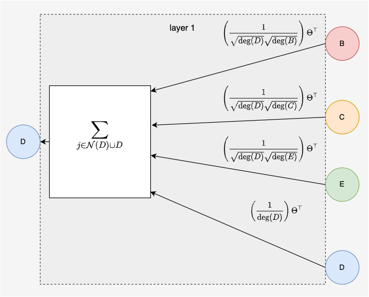
We can look at the first layer of the GCN to see how it passes messages. Each node vector is multiplied by a weight matrix $\boldsymbol{\Theta}^{\top}$ and then normalized by the product of degrees. This normalizing will prevent message vectors from exploding and it will remove degree bias.

Graph Attention Network (GAT)

Message Passing View

$\mathbf{x}_i^{\prime}=\alpha_{i, i} \boldsymbol{\Theta} \mathbf{x}_i+\sum_{j \in \mathcal{N}(i)} \alpha_{i, j} \boldsymbol{\Theta} \mathbf{x}_j$ $\alpha_{i, j}=\frac{\exp \left(\operatorname{LeakyReLU}\left(\mathbf{a}^{\top}\left[\boldsymbol{\Theta} \mathbf{x}_i \| \boldsymbol{\Theta} \mathbf{x}_j\right]\right)\right)}{\sum_{k \in \mathcal{N}(i) \cup\{i\}} \exp \left(\operatorname{LeakyReLU}\left(\mathbf{a}^{\top}\left[\boldsymbol{\Theta} \mathbf{x}_i \| \boldsymbol{\Theta} \mathbf{x}_k\right]\right)\right)}$
$||$ - Concatenation

$\Theta$ - Weight matrix. This is the same matrix in both $\mathbf{x}^{\prime}_i$ and $\alpha_{i,j}$ equations.

$\mathbf{a}$ - Attention weights

$\alpha$ - Attention weight matrix

Matrix View

$X^l = \sigma(\alpha AX^{(k-1)}\boldsymbol{\Theta})$

The Graph Attention Network (GAT) was first published later in 2017 by Petar Veličković. The GAT looks just like the GCN but it replaces the normalizing factor with an attention mechanism. Intuitively the attention weights will amplify important edges and suppress unimportant edges for the given prediction task³.

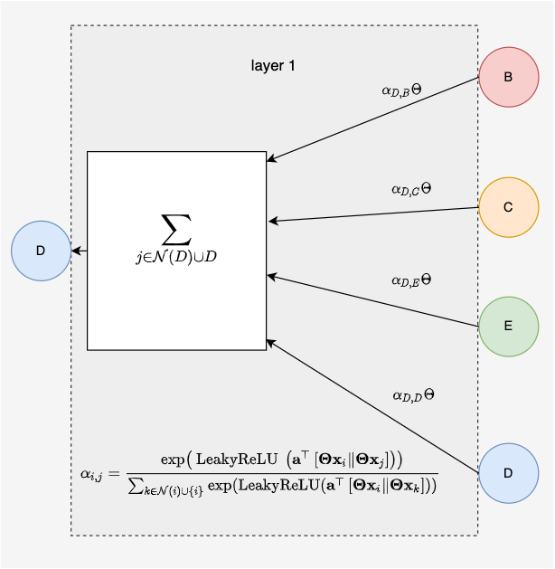
The attention mechanism was made famous in the transformer paper that used a pair wise attention across the entire input vector⁴. Sometimes the attention mechanism applied to GAT is called masked attention, because it only considers edges within the underlying graph, "masking" or zeroing out all other attention coefficients³.

Attention weights are computed as a softmax of learned attention coefficients giving a value ranging from 0 to 1 for each attention weight in the attention matrix $\alpha$ . The sum over any given row or column will be 0. The attention matrix $\alpha$ can be seen as weighted adjacency matrix where each of the non-zero elements is an attention weight. This maps on nicely to the matrix view of GAT.

For an in depth explanation see Understanding Graph Attention Networks on YouTube or check out the original Graph Attention Networks Paper.

Graph Isomorphism Network (GIN)

Message Passing View

$\mathbf{x}_i^{\prime}=h_{\Theta}\left((1+\epsilon) \cdot \mathbf{x}_i+\sum_{j \in \mathcal{N}(i)} \mathbf{x}_j\right)$
$\epsilon$ : Hyperparameter that varies the impact of the self-loop.

$h_{\Theta}$ : A neural network, .i.e. an MLP.

Matrix View

$X^l = h_{\theta}(\sigma(X^{(k-1)}))$

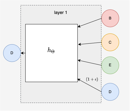
The Graph Isomorphism Network (GIN) is a more complex version of the GCN that was published in 2019 by Keyulu Xu et al⁵. This idea can be rationalized by the universal approximation theory of neural networks that shows nearly any function can be approximated by a two layer neural network ⁶ $^,$ ⁷. By passing the node representations through multiple layers of a Multi-Layer Perceptron (MLP) the GIN is more complex in number of parameters but more expressive in in the data distributions that can be learned.

§ GIN Theory

Graph Kernels

Graph kernels are used to compute the similarity between two graphs. $\phi$ is used to map $G$ to a different space then similarity is computed in that space as the inner product $\phi({G})^{\top}\phi({G^{\prime}})$ . Graph kernels are one of the traditional methods used for learning on graphs.

Weisfeiler-Lehman(WL) Kernel ¹

The Weisfeiler-Lehman (WL) Kernel is a popular kernel for its time complexity and because of its expressiveness which is the ability to distinguish a large number of different types of graphs. WL Kernel computes computes $\phi$ via the color refinement algorithm.

Color Refinement Algorithm:

Given a graph $G$ with a set of nodes $V$

Assign an initial color $c^{(0)}(v)$ to each node $v$

Iteratively refine node colors by

$C^{(k+1)}(v)=\operatorname{HASH}\left(\left\{c^{(k)}(v),\left\{c^{(k)}(u)\right\}_{u \in N(v)}\right\}\right)$

$\operatorname{HASH}$ maps different inputs to different colors

After $K$ steps of color refinement, $c^{K}(v)$ summarizes the structure of the $K$ -hope neighborhood.

The $\phi$ from the WL kernel counts the number of nodes of a given color. $\phi$ represents a graph with a bag of colors. In more detail the kernel uses a generalized version of "bag of node degrees" since the node degrees are one-hop neighborhood information.

The WL kernel provides a strong benchmark for the development of GNNs since it is both computationally efficient and expressive. The cost to compute the WL kernel is linear in the number of edges since at each step information is aggregated at each node from its neighbors. Counting colors is linear w.r.t. the number of nodes, but since there are typically an order magnitude or more edges than nodes in real world graphs, the WL kernel time complexity is linear in the number of edges. Since we are discussing the kernel this is number of edges in both graphs.

WL Graph Isomorphism Test

The WL Graph Isomorphism Test (WL test) only guarantees that two are graphs not isomorophic if $\phi{(G)}^{\top}\phi{(G)} \neq \phi{(G)}^{\top}\phi{(G^{\prime})}$ , at any stage during color refinement. In general the WL test can give a measure of similarity or closeness to isomorphism between two graphs.

WL Test Toy Example

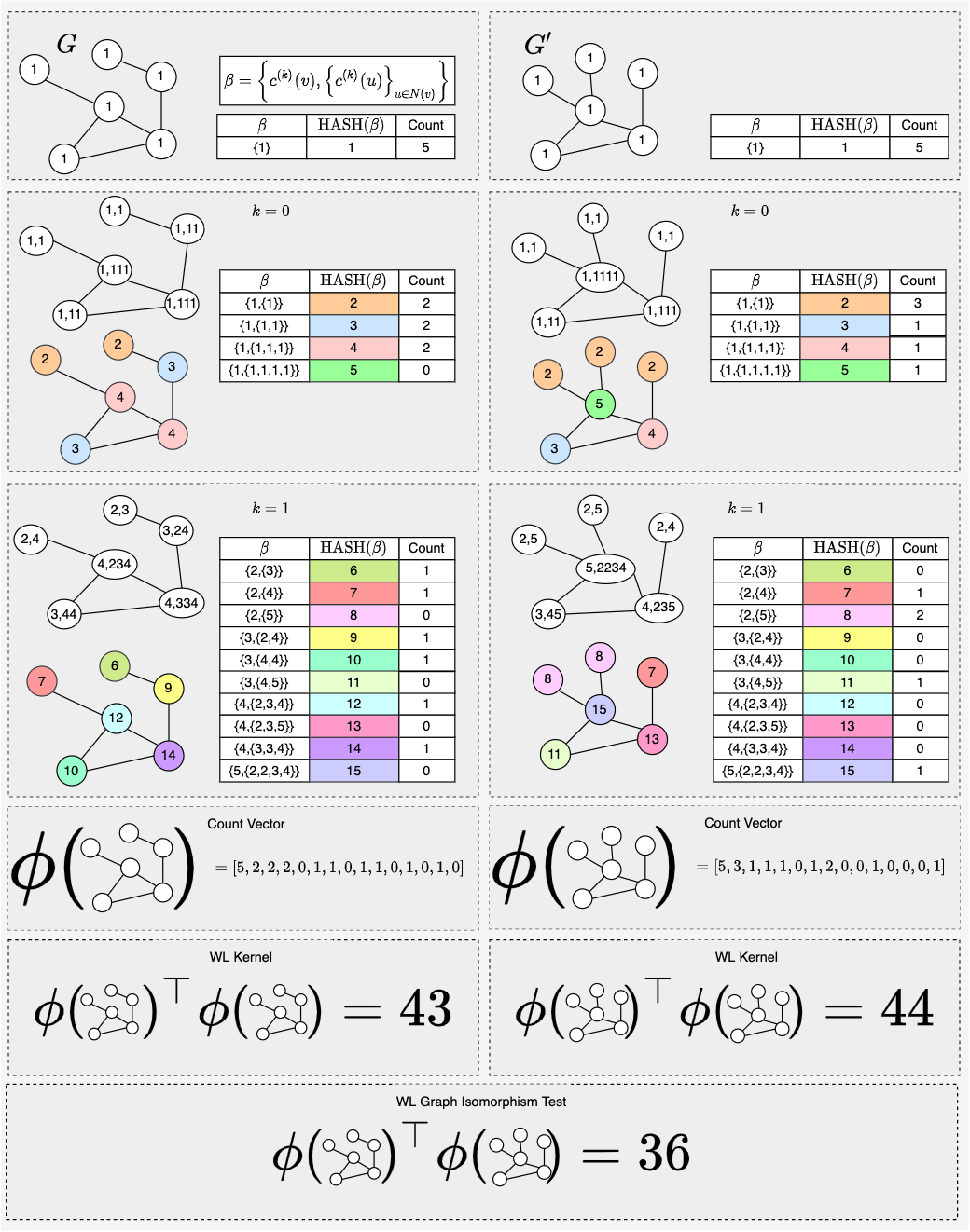
As we can see in the example different colors capture different $k$ -hop neighborhood structure. In this case $\phi({G})^{\top}\phi({G^{\prime}})=36$ . We know from $\phi({G})^{\top}\phi({G})$ and $\phi({G^{\prime}})^{\top}\phi({G^{\prime}})$ , that the two graphs are not isomorphic. In fact, we could have seen that these graphs were different after the first stage of color refinement.

Graph Isomorphism Network

In How Powerful are Graph Neural Networks, the GIN is proven to be at least as expressive as the WL test, whereas the GCN is shown to worse than the WL test in some cases².

§ Experiments

Models

To test the hypothesis that the GIN is more expressive we trained a GCN, GAT, and GIN model on a benchmark dataset provided by OBG. The models are trained and then nodes representations are pooled to get a global representation of the graph for graph classification. All source code for the models can be found in the pyg_gym directory. Specifically the following files are used to train models:

OGB Data

To familiarize yourself with the dataset we recommend reading the description of obgb-ppa. I have copied the relevant row from the data table provided. In brief, this is a graph classification tasks over 37 different classes.

Scale	Name	Package	Num Graphs	Num Nodes per graph	Num lEdges per graph	Num Tasks	Split Type	Task Type	Metric
Medium	ogbg-ppa	>=1.1.1	158,100	243.4	2,266.1	1	Species	Multi-class classification	Accuracy

Wandb

All experiments can be viewed on wandb. This workspace should be public access so comment below if it is not.

At the time of last commit, models were still in the process of training so I did not pull in their key results.

§ Future

Compare GCN and GIN with the WLConv, which equivalent $\phi$ of the WL-kernel.
Run GCN and GIN over some small graphs where they are known to have different theoretical results. Showing these models can be trained and that they match theory will help build intuition around matching theory to experiment.